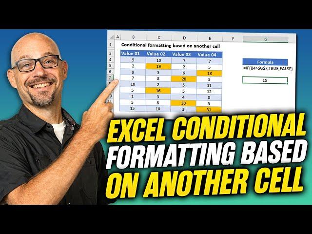
Excel How To: Format Cells Based on Another Cell Value with Conditional Formatting

This helped for what I was looking for. Gracias! :)

Create a column of values you want to use as your references, color code and group your cells in this column accordingly, but don't go too crazy with it.

Create a second column, and input the data validation into your first cell of the new column, selecting the first column as your list. With the cell containing your data validation still selected, open conditional formatting, create a new rule, and set it to determine what to format based on a formula; input and update the following formula with the actual values for your table: =VLOOKUP($ColumnRow,$Column$Row:$Column$Row,1,TRUE)=$ColumnRow

Depending on how many groups you have in the reference column, you will need to duplicate this rule manually for each one. If you only want to reference a single cell for formatting, remove the ":$Column$Row" in the range portion of the formula, or use a simpler formula. This is why I said not to go too crazy with the formatting: For each rule, mirror the formatting of the group/cell to which it pertains. Click OK.

In the box next to each rule that is labeled "Applies to", enter the range of cells you're going to need the list populated in. If my list is in cells E4 to E80, it should read =$E$4:$E$80. Click Apply.

There you go; just saved you two hours of troubleshooting formulas yourself if that's what you were looking to do like I was when I came upon this video.

you are the best!!!!! Thanks!

I’m putting this in here for others as I fought with my formula not working for about an hour.
If you’re using true/false for highlighting it won’t work with quotes as the Boolean terms of true/false don’t need quotation marks.

wow- thanks a ton

I want to be able to highlight a blank cell that has a formula. So my simpler second sheet is fed from the first by having a formula (eg =Sheet1!A1), but because there is a formula this does not work even though sheet1 cell A1 has no data. Help please?

That explanation technique was just WOW!

Great explanation - exactly what I needed. Thankyou!

Thanks!

Is there a way to do this but in a Pivot Table and using the source data for the conditional formatting?

This is a great video. I'm using a Data Validation drop down list (Sheet 1) where I select a customer name from my database (Sheet 2). I'd like to apply this video's conditional formatting but rather than highlight the row(s) on Sheet 1 - where my data validation and vlookup formulas are located, I'd like it to back to my database (Sheet 2) and highlight the rows of the customer names, that I've selected on Sheet 1. What do I need to change/add to Excel Universities formula to accomplish this? Thank you!

Halleluia!!! Finally, I've found a video which explained the mechanism behind conditional formatting. I managed to make a formula that I needed, being a total beginner. I made a drop-down list in row B, and wanted to highlight cells in row A depending on the chosen text from the list in row B. This video has made this possible. Thank you and liked and subscribed!!!

You made me looks the smartest in front of my boss..thanks too much bro

Very nice video, may I ask one question?
How can we protect columns dynamically while using conditional format OR Can we lock cells with conditional format dynamically with out VBA?

Wonderful, you helped me do something I have been trying for ages how to get a line formated when the date (in column A) is today - =$A2=TODAY()

Can you create a formula that takes into account only columns that contain a certain word? For example, is it possible to create a sum of the “amounts” marked as open?

Can you please do a video on how to highlight the whole row is only some cells are highlighted (N.B : but the cells are not common)

Thank you so much! It solved the problem I was having at work. I used to spend lots of time highlighting rows. All of your videos are super helpful.<3

Although I use advanced sheets for years, the way you explained Cond. Form. makes possible to understand the concept behind the logical thinking, like a programmer. After that I made some tests on a huge sheet and I could notice a new level of control of the conditional formatting. You made simple something no one could explain so clearly before. Congratulations!

How do I apply conditional formating to a check box where the box being checked applies the formula?

Excellently explained and has really helped me with a work project. Thanks!

Thank you, Thank you, Thank you! Explained so simply.

Good explanation!

Thank you very much for this video and information! Nice Explanation!!👌👌👌

Super helpful and explained well!

i want to use conditional formatting if any value changes in that cell not relative to another cell

Solved my problem. Thanks!

Thanks Paul

Explained everything really well, easy to follow, great teaching technique.

Amazing m!! Looking to format a large amount of data but am struggling to figure out the best formula suitable for formatting a time scale set of data. Needs to read value of each set of data on each row by itself if this makes sense.. so Tiring 😢

Really well explained and so simple - thank you

Thanks for explaining this so thoroughly, yet slow enough to make sense. I can see myself watching a LOT of your videos in the near future!

I have seen many excel teaching videos.. I can honestly say, you know how to teach. Awsome channel.

Awesome! thanks

Thank you, may God bless you

You explained this so well, thank you for taking time to explain vs. simply sharing the formula.

I want data depending on cell status i have Active and Closed. So i have data in A,B and in C i have Active or Closed, So If i select Closed then data in A,B should add up and be displayed in column D, how can we do it?

struggling to get this to work with cells already containing data validation.

I want to create a drop down list wherein Column A (with validation) will format to maintain the same colour of Column B (data validation). Column b13 takes validation from a list in column X, and conditional colours of its own for text containing specific phrases "Phrase A" "Phrase B" etc

when I use the formula: =$b13="Text Phrase"

I'm getting no results in A13. verified that "apply selection to" says A13.

feeling lost, please help if possible.

Great video. Can you use wildcards in your formula? I am trying to conditionally format certain cells based on one cell having data in it, but that data changes every row that I want to format and cells in between don't have data in that cell.

Great overview - seriously good. Nice work boss.

hi, can we do format cells based on different sheet ?

Is it possible to add data to an existing Table(Calender)? I have a calender but would like to have data from a different workbook(s) automatically enter into dated cells.

You are a good teacher. Thank you.

This is extremely helpful, thank you so much!

Thank you very much for this video and information! Exactly what I was looking for in working on my own projects. Well put together video and very informative.

obsessed with soft design now and more obsessed with cool scales Nd stuff.

Well presented Sir !!!! Nice video

Nice tutorial Michael,